Validating Assumptions and Remediation

[A, SfS] Chapter 8: Correlation and Regression: 8.3: Validating Assumptions and Remediation

Validating Assumptions and Remediation

Validating Assumptions and RemediationIn this section, we will discuss how we can check that the assumptions for the linear regression model have not been violated. Additionally, we will discuss how to salvage the model, in case there is a violation of one of these assumptions.

All of the statistical inference conducted in linear regression depends on the validity of the assumption that the residuals represent a random sample from a normal distribution with mean #0# and a variance #\sigma^2# that does not depend on the value of the independent variable (i.e., the residuals are homoscedastic). The validity of this assumption must be checked.

Residual Plot
One important diagnostic tool is a plot of the residuals #e_1,...,e_n# against the fitted values #\hat{y}_1,...,\hat{y}_n#, called the residual plot.

Ideally, the residual plot will show a random scatter of points within a horizontal band of constant width, with no evident pattern, centered at zero.

For example:

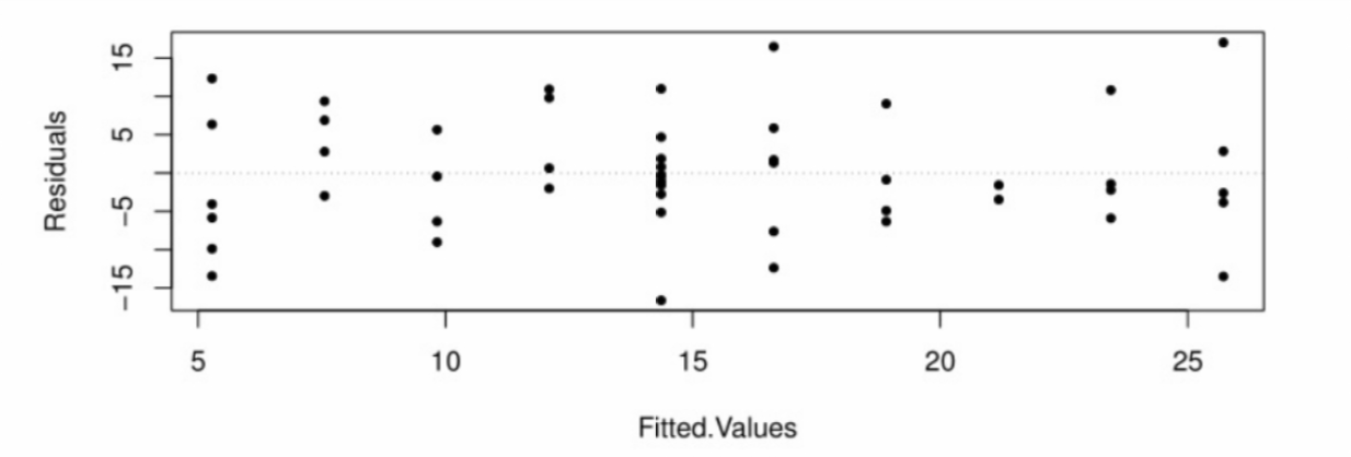
Here we see that the points are scattered between #-15# and #15# across the full range of the fitted values, with no pattern showing. Although this tells us nothing about whether or not the assumption of normality is valid, it does show that the variance of the residuals does not appear to depend on the value of the independent variable, i.e., that we have homoscedasticity.

Moreover, that absence of a pattern allows us to conclude that the linear model is an appropriate choice. We can also see that there are no outliers among the residuals. If there had been one residual with a value outside the #(-15,15)# range, e.g., a value of #25#, we would be concerned about the influence of that measurement on the model fit.

In contrast, the following residual plot shows clear evidence of heteroscedasticity: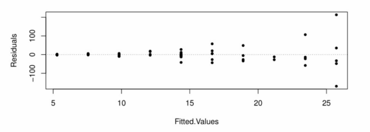

Here we see that the vertical spread of the residuals grows larger as the fitted values increase, which makes it obvious that the variance is not constant, but depends on the value of the IV. This invalidates any statistical inference we might make about the regression model.

In the above plot, we see that there is a correlation between the magnitude of the residuals and the fitted values, i.e., the larger the fitted value, the larger the average magnitude of the residuals. So we could assess a departure from the homoscedasticity assumption by performing a test for a non-zero correlation coefficient between the squared residuals and the fitted values. In this case, we would not want to reject the null hypothesis that the correlation coefficient equals zero.

A residual plot can also be useful to identify when the linear model is not appropriate. The next residual plot shows what happens when a line is used to model data from a non-linear relationship: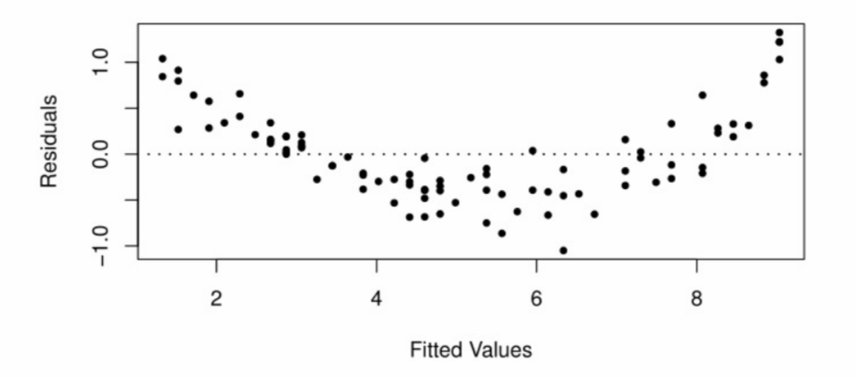
The non-linearity becomes magnified in a residual plot. This is a clear signal that a linear model should not be used. However, this problem should already have been visible in a scatterplot of the DV against the IV.

Outliers are also visible in the residual plot as well as in the original plot of the DV against the IV. In a large data set it is reasonable to have a few outliers, but one should nevertheless decide whether or not to delete such cases from the data set.

One criterion for consideration is whether or not the outlier is an influential point, i.e., if deleting it has a dramatic effect on the least-squares estimates of the slope and intercept. If not, then it is best to leave it in the data set.

\[\text{}\]One assumption that cannot be checked with the residual plot is the assumption of normality of the residuals. To check the validity of this assumption, one can use the normal quantile-quantile (Q-Q) plot for the residuals.

Normal Quantile-Quantile PlotThe normal quantile-quantile (Q-Q) plot for the residuals is a scatterplot created by plotting the quantiles of the residuals against the theoretical quantiles of the standard normal distribution.

If the assumption of normality of the residuals holds, we should see the points form a roughly straight line.

The following Q-Q plot of the residuals shows a good match between the quantiles of the residuals and the theoretical quantiles of the standard normal distribution: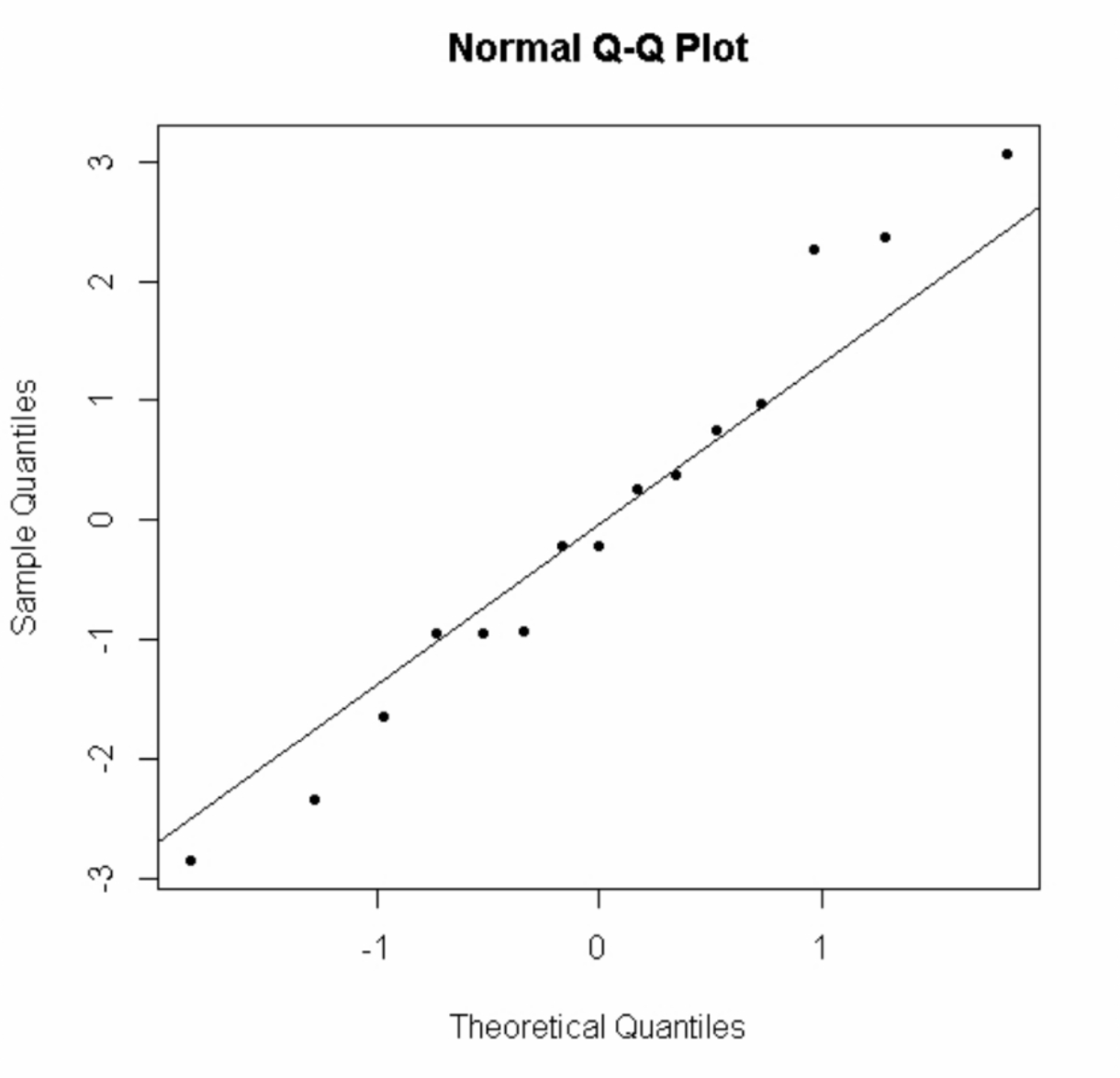

One can also conduct a hypothesis test such as the Shapiro-Wilk test for normality, in which the null hypothesis is that the residuals are normally distributed.

The assumption of independent observations relies on whether the data collection was done properly, using random sampling from the population. However, if the data were collected over time, one could plot the residuals against the time order of the data collection. If a pattern is visible, then the independence assumption is violated.

\[\text{}\] If violations of the assumptions are detected, remedial measures should be considered. One technique is to transform the data, either the IV or the DV or both.

For example, if the scatterplot shows a curved trend that appears to be exponential, then a better model for the association between #Y# and #X# would be: \[Y = \beta_0e^{\beta_1x}\]

This can be transformed into a linear model by taking the logarithm of both sides: \[\ln Y = \ln \beta_0 + \beta_1x\]

Then in the data set, create a new dependent variable #W# in which you compute the logarithm #W = \ln Y# for each case (assuming all values of the DV are positive), and then proceed with a linear model with #W# as the DV and #X# as the IV in order to estimate the intercept #\ln \beta_0# and the slope #\beta_1#.

One can then exponentiate if necessary to transform the linear model back into an exponential model.

Other possible examples of transformations include power transformations and square root transformations. There is no guarantee that a transformation will remediate problems with the assumptions, but quite often a clever transformation will succeed.

Alternatives to transformations include multiple regression, polynomial regression, weighted least-squares, and nonlinear regression. We will only learn about multiple regression in this course. \[\text{}\]

Using RResidual Plot

To make the residual plot, after you have already fit a linear model to the data (assuming you have named the model as Model):

> plot(Model$fitted.values, Model$residual, pch=20, main="Residual plot", xlab="Fitted values", ylab="Residuals")

> abline(h=0, lty=3)

Homoscedasticity Assumption

The homoscedasticity of the residuals can be checked formally by testing for a non-zero correlation between the squared residuals and the fitted values. In this case, the null hypothesis is that there is no correlation, which implies homoscedasticity, so you would want a large P-value for this test. In #\mathrm{R}#:

> cor.test(Model$residuals^2, Model$fitted.values)

Q-Q Plot

To make a Q-Q plot of the residuals:

> qqnorm(Model$residuals, pch=20, main="Q-Q plot of the residuals")

> qqline(Model$residuals)

Normality Assumption

The normality of the residuals can be checked formally using the Shapiro-Wilk test, for which the null hypothesis is that the residuals come from a normal distribution. Hence you would want a large P-value for this test. In #\mathrm{R}#:

> shapiro.test(Model$residuals)