Operations with complex numbers: Calculating with complex numbers
 Imaginary numbers
When studying quadratic equations, we found out that not all of them have roots. This is true if we restrict ourselves to real numbers, but not when imaginary numbers are introduced, and we allow for so-called complex solutions, which will be defined later.
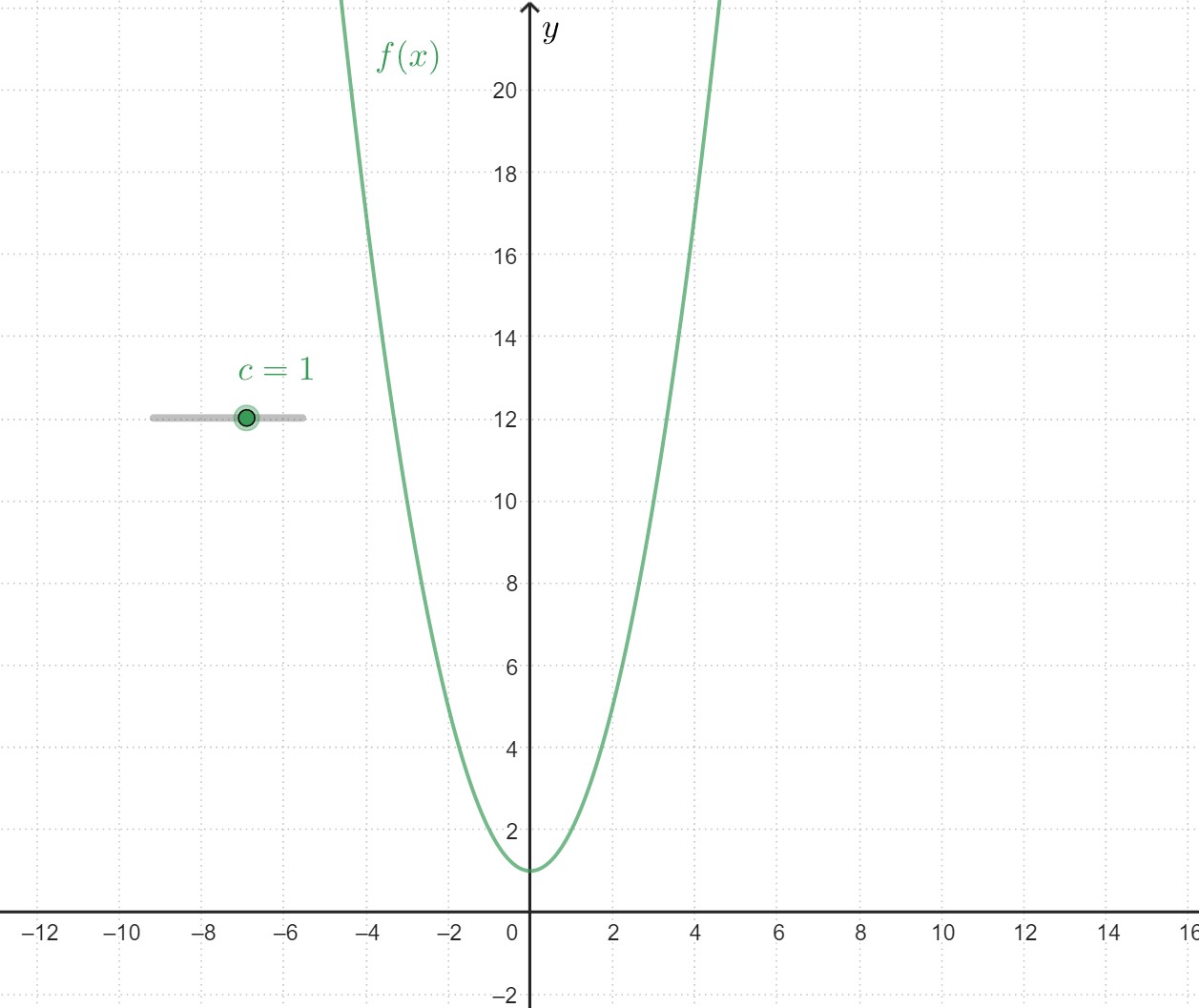
Consider an equation of the type \[x^2+\green{c}^2=0\] where #\green{c}# is a real number. This equation has no real solution, unless #\green{c}=0#. Because
\[\begin{array}{rcl} x^2&=&\displaystyle -\green{c}^2\\&&\quad\blue{\text{subtracted }c^2\text{ from both sides}}\\
x&=& \pm\sqrt{\displaystyle -\green{c}^{2}}\\
&&\quad\blue{\text{took the square root of both sides}}
\end{array}\]
which is not possible for real numbers #\green{c}\neq 0# as #\green{c}^2>0#, meaning #-\green{c}^2<0# and there are no real square roots of negative numbers.
However, as we will see in this chapter, if we allow #x# to have an imaginary part, then the equation #x^2+\green{c}^2=0# has solutions.
Imaginary numbers are numbers whose square is negative. In the same way that real numbers have a unit in the number #1#, imaginary numbers have their unit in #\blue{\complexi}#, a number which is defined to be such that #\blue{\complexi}^2=-1#.
The imaginary unit is written as #\blue{\complexi}# and it is a number whose square equals #-1#,\[\blue{\complexi}^2=-1\]
This means that \[ \blue{\ii} = \sqrt{-1} \]
By multiplying #\blue{\complexi}# with real numbers, we obtain imaginary numbers.
An imaginary number #\purple{y}# has the general form \[\purple{y}=\green{b}\cdot \blue{\complexi}\] where #\green{b}# is a non-zero real number.
The following are imaginary numbers: \[\begin{array}{rc}
&\purple{y}=\green{2}\cdot\blue{\complexi}\qquad\qquad
\purple{y}=\green{\sqrt{3}}\cdot\blue{\ii}\\
&\purple{y}=\green{-\cfrac{10}{3}}\cdot\blue{\complexi}
\qquad\qquad\purple{y}=\green{-\cfrac{\pi}{6}}\cdot\blue{\complexi}\end{array}\]
One of the most interesting properties of #\blue{\complexi}# emerges when we take successive powers of the imaginary unit. Using that #\blue{\complexi}^2=-1#, we can derive rules for this.
The results of taking successive powers of #\blue{\complexi}# cycle between #1#, #\complexi#, #-1#, and #-\complexi#.
General case
\[\begin{array}{rcl}
\displaystyle\blue{\complexi}^{\orange{4n}}&=&1 \\
\displaystyle\blue{\complexi}^{\orange{4n+1}} &=& \blue{\complexi} \\
\displaystyle\blue{\complexi}^{\orange{4n+2}} &=& -1 \\
\displaystyle\blue{\complexi}^{\orange{4n+3}} &=& -\blue{\complexi}
\end{array}\]
where #\orange{n}# is an integer.
Examples
\[\begin{array} {rclcrcl}
\blue{\ii}^{\orange{0}} &=& 1 &\text{ }& \blue{\complexi}^{\orange{4}} &=& 1 \\
\blue{\complexi}^{\orange{1}} &=&\blue{\complexi} &\text{ }& \blue{\complexi}^{\orange{5}} &=&\blue{\complexi}\\
\blue{\complexi}^{\orange{2}} &=&-1&\text{ }& \blue{\complexi}^{\orange{6}} &=&-1\\
\blue{\complexi}^{\orange{3}} &=&-\blue{\complexi} &\text{ }& \blue{\complexi}^{\orange{7}} &=&-\blue{\complexi} \\
\end{array} \]
The usual rules of exponentiation apply to #\blue{\complexi}# as well, for instance, #\blue{\complexi}^{\orange{0}}=1# and #\blue{\complexi}^{-\orange{n}}=\frac{1}{\blue{\complexi}^{\orange{n}}}#.
Non-integer powers of #\blue{\complexi}# will be discussed later in the broader context of complex exponentiation.
As we saw in the example of the quadratic function, some real quadratic equations cannot be solved because there are no real square roots of negative real numbers. However, we can construct imaginary square roots of negative real numbers.
Let #\green{a}# be a positive real number. Then, the square root of #-\green{a}# can be expressed in terms of #\blue{\complexi}# as
\[\begin{array}{rcl}
\displaystyle\sqrt{-\green{a}}&=&\displaystyle\sqrt{\green{a}}\cdot\blue{\complexi}
\end{array}\]
Examples
\[\begin{array}{rcl}
\sqrt{\displaystyle-\green{7}}&=&\displaystyle\sqrt{\green{7}}\cdot\blue{\complexi}\\
\sqrt{\displaystyle-\green{4}}&=& \displaystyle\green{2}\cdot\blue{\complexi} \\
\sqrt{\displaystyle-\green{36}}&=&\displaystyle\green{6}\cdot\blue{\complexi}
\end{array}\]
Recall that #\,\complexi^4=1#. Using this information and the rules of exponentiation, we obtain
\[\begin{array}{rcl}
\complexi^{8} &=& \complexi^{4+4} \\
&&\quad\blue{\text{wrote }8 \text{ as }4+4} \\
&=& \complexi^4 \cdot \complexi^4 \\
&&\quad\blue{\text{used exponentiation rule }\,a^{b+c}=a^b\cdot a^c}\\
&=& 1 \cdot 1 \\
&&\quad \blue{\text{substituted } \,\complexi^4=1} \\
&=& 1 \\&&\quad \blue{\text{simplified}}
\end{array}\]